Open Cluster Candidate Detection Using DBSCAN
Alex | Last updated: May 19, 2019
Open clusters are groups of generally—though not necessarily—young stars found in the galactic plane. The stars are bound by gravity and share similar ages, chemical compositions, and positions in space.
In many respects, open clusters are gateways to understanding interesting astrophysical topics such as stellar formation, stellar evolution, stellar dynamical interactions, galaxy evolution, and so forth. However, to study such interesting astrophysics using open clusters, one must first be able to detect open clusters.
With the Gaia Data Relase 2 (Gaia DR2), we now have positional and kinematic information for over one billion stars. Machine learning techniques promise efficient ways to process and investigate the catalogue for trends and discoveries.
This project followed a machine-learning method of open cluster candidate detection proposed by Castro-Ginard et al.The associated paper, Castro-Ginard et al. (2018) (arXiv) discusses both the detection of stellar cluster candidates and their classification into confirmed clusters versus false positives. I focused on replicating the detection portion of their proposed data process.
The proposed data processing method promises automation—instead of manually cutting positons, parallaxes, and proper motions, the paper proposes basic statistical preprocessing of Gaia data before using an unsupervised learning algorithm, DBSCAN, to detect overdensities in select astrometrical parameters. Detected overdensities are considered signals of star cluster candidacy that would prompt further investigation.
Finding Clusters Naively
One method of finding clusters is to simply “draw” a cylinder in the sky, perform some data cuts, and call it a day:
- “Point” the telescope at select coordinates in the sky using
SkyCoord. - “Draw” a circle of radius 3 degrees around the selected coordinates with
astroquery. - Query Gaia DR2 for data points containing “good” measurements of RA, Dec, Parallax, stellar proper motions, stellar parameters (e.g. color and effective temperatures), and their associated errors.
- Clean data by removing data points with large error values and filtering for data points with several visibility periods.
- Perform data cuts by restricting the queried sample to the literature distancesfrom the the centers of our clusters; select for stars that are within 10 pcs of reported cluster center coordinates.
Example: The Hyades
To demonstrate this method, I wrote a SQL query that effectively “pointed” the telescope at and “drew” a 3-degree radius circle around select coordinates in the sky with a known star cluster: the Hyades.
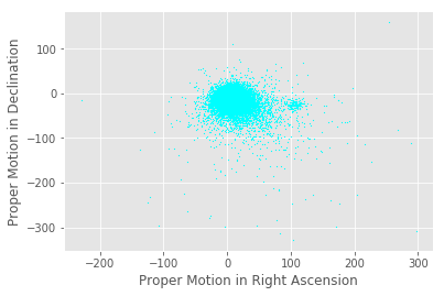
To perform data cuts using distance, I converted the desired distance range into parallax angles with a naive estimate:
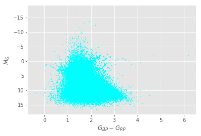
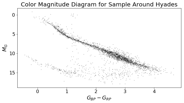
I then used the distance modulus to obtain an absolute magnitude G-band value from the apparent (measured) G-band magnitude the previously calculated distance values. With absolute magnitude, we can plot a color-magnitude diagram.
As a sanity check, I superimposed a HIST-generated isochrone, assuming a log age of 8.796, a metallicity of +0.2, and an interstellar extinction av value of 0 (because the Hyades is relatively close to us).
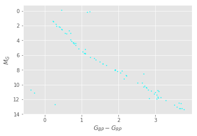
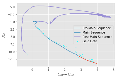
So this method works… sort of. We get a reasonable color-magnitude diagram that fits well with a model isochrone.
The advantage of the cylinder method, however clunky, is its simplicity: the approach leverages basic astronomy concepts (the distance-paralllax formula and the distance modulus) and requires only simple data cuts to estimate cluster membership.
The problem, however, is that this approach works for finding known clusters—we need to know the coordinates representing the center of a cluster beforehand. It’s more cluster selection than it is detection Moreover, the approach does not account for various factors such as errors in measurement, astrophysical phenomena such as dust scattering light (which would introduce massive errors in distance calculations), and so on.
One might think of using machine learning and statistical inference with this approach—for instance, find data that “fits” theoretical isochrones—but this is computationally expensive and unreliable—it amounts to brute force guessing that involves only performing an arbitrary number of distance cuts on an arbitrary number of coordinates, but also fitting an arbitrary number of isochrones that can be generated with an arbitrary number of parameters.
Honestly, that kind of sounds like machine learning in research in a nutshell. But we can do better.
DBSCAN
DBSCAN stands for “Density-Based Spatial Clustering of Applications with Noise.” It is an unsupervised learning algorithm that is ideal for large samples and does not rely on any underlying assumptions about the dataset—which makes it flexible and capable of discovering clusters of arbitrary shapes.
DBSCAN finds clusters based on overdensities, or high-density regions in the data. A high-density region is defined by two parameters:
- , the distance between cluster members—often denoted as
Rfor radius. Points are “reachable” from one another if they lie within distance from each other. - , the minimum number of points for a neighborhood of radius—often denoted as
Mto be considered a cluster.
A hypersphere of radius is built around each data point in the parameter space, and the set of points that fall within the hypersphere is considered “dense”—a cluster—if the number of points exceeds minPts.
DBSCAN clustering generates three types of points:
- Core points: Points that have at least
minPtsneighbors within distance from themselves. - Member points: Points that don’t have
minPtsneighbors within their hyperspheres, but fall within the hypersphere of a core point. - Noise points: Points that are neither Core nor Member points—generally considered outsliers.
K-Means Clustering
K-means is one of the most popular clustering methods in machine learning. The algorithm is an example of partition-based, unsupervised learning and involves repeating iterative steps:
- Initialize
kcentroids to be randomly placed in the parameter space of interest. - The distance between each data point from each centroid is calculated.
- Each data point is assigned to its closest centroid—the resultant assignments represent clusters.
- The
kcentroids have their positions recalculated in the parameter space—until they represent means, hence the name of the algorithm.
With K-Means clustering, a data point is considered a member of a particular cluster if it is closer to one centroid than it is to any other centroid.
DBScan vs K-Means
| DBSCAN | K-Means |
|---|---|
|
|
Given the noisiness and propensity for error and outliers in astrophysical measurements, as well as the lack of a prior k value, DBSCAN is a natural choice when it comes to stellar cluster detection.
Using DBSCAN to Detect Star Clusters
To apply the DBSCAN algorithm to detect open clusters in the parameter space of astronomical data, Castro-Ginard et al. propose the following procedure:
- Define the search region.
- Perform data “normalization.”
- Determine the average distance between stars in parameter space.
- Determine and
minPtsfor DBSCAN, which the researchers propose a method to. - Set
ktominPts - 1, sinceminPtsdetermines the minimum number of members needed for a set of points to be considered a cluster. - Use DBSCAN for overdensity detection with and
minPtsas parameters and and using distance metric on standardized values.
Defining Our Search Region
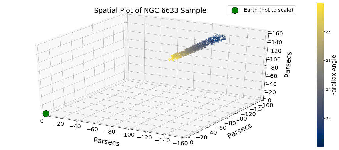
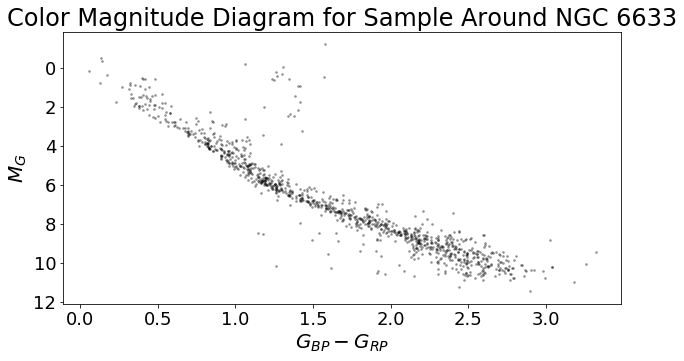
I used SkyCoord from astropy to select coordinates (ICRS) for known clusters and astroquery to query Gaia DR2 for the stellar population in selected regions around the coordinates (within 1 degree of the “center” coordinate).
I choose to use the same example the paper uses to demonstrate how their method works when applied to a star cluster: NGC 6633, a star cluster that is roughly 350 parsecs away.
- I treated the reported coordinates as the center of the cluster and queried for a parallax region that is 50pc behind (400 pc away) and 50pc (300 pc away) in front of that distance.
- I queried for objects that are in the Galactic disc () and filtered out objects with extreme proper motions and large/negative parallaxes (reject stars with the following values: , mas yr−1, , mas and mas).
Data Normalization
I first processed the queried data using scikit-learn’s implementation of the Yeo-Johnson power transformation. The power transformation “normalizes” the data points to make our sample look and behave more Gaussian and reduce the effects of outliers.
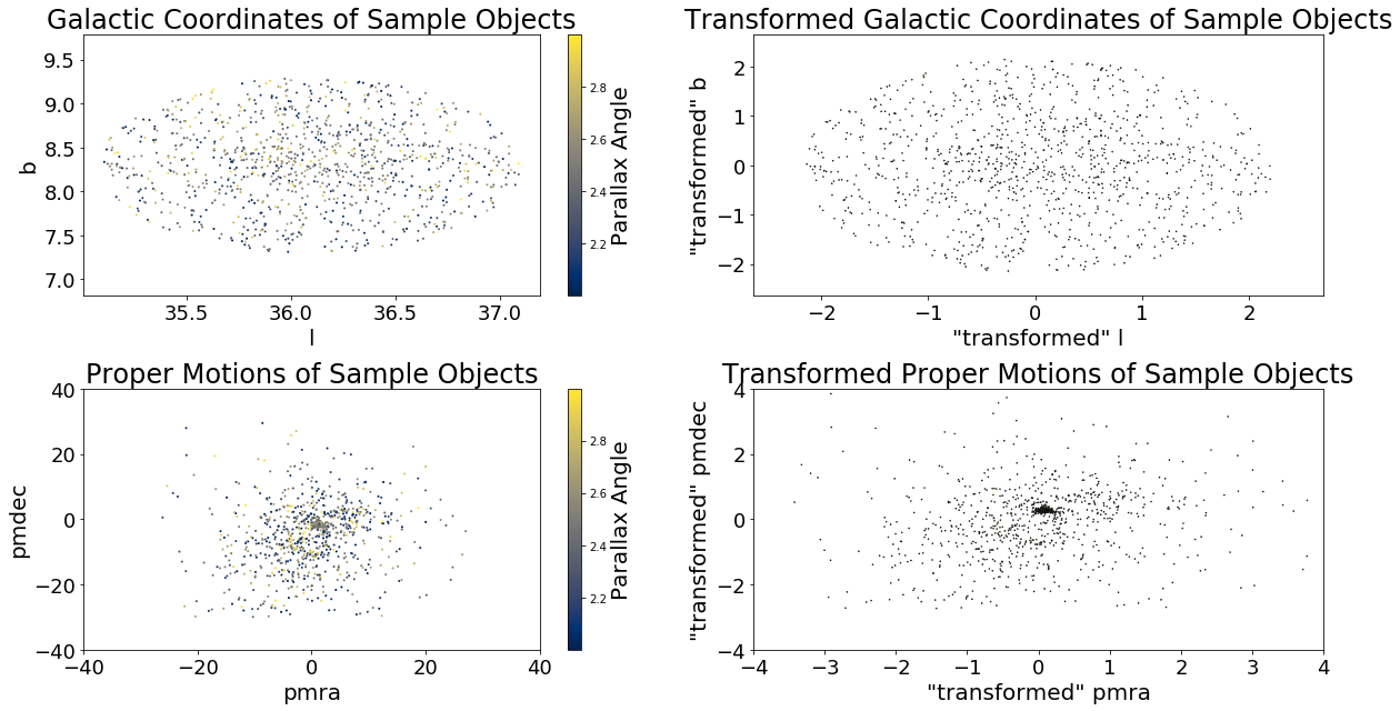
Once the data has been processed, we can follow the instructions provided Castro-Ginard et al. (2018).
Determining Mean Distances Between Points
The authors propose using a Euclidian distance metric that computes pairwise distances between standard points using galactic coordinates, parallax angles, proper motion measurements:
This distance metric is simple to understand and easy to use, so we use this for a naive first-pass using DBSCAN.
Compute
To compute , the authors propose a procedure:
- Compute the Nearest Neighbour Distance () histogram for each region and store its minimum as . (The kNND is the distance from each point to its kth nearest neighbor)
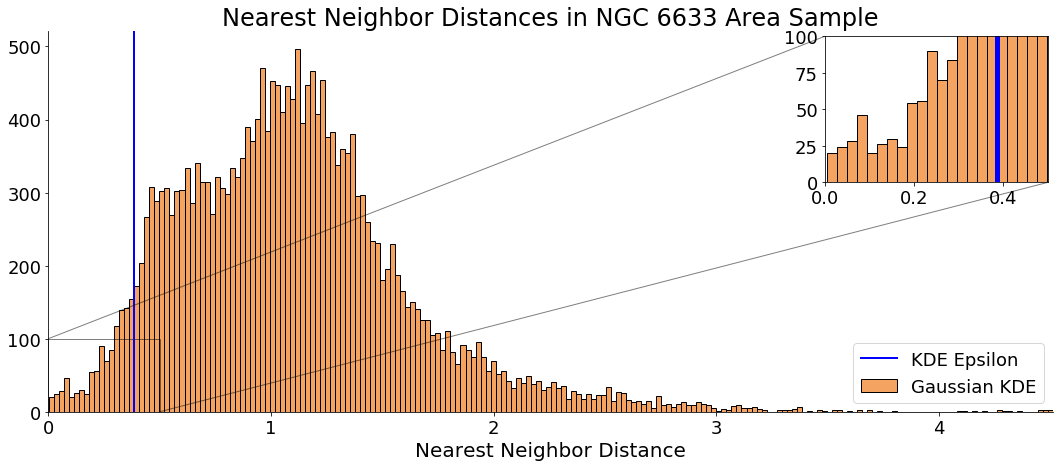
- Generate a new random sample, of the same number of stars, according to the distribution of each astrometric parameter estimated using a Gaussian kernel density estimator. Then, compute the histogram for these stars and store the minimum value as . Since we are generating random samples, the minimum number of the distribution will vary at each realization, in order to minimize this efect we store as the average over 30 repetitions of this step.
- Finally, to get the most concentrated stars and minimize the contamination from field stars, the choice of the parameter is
By “store its minimum as ,” it seems the authors meant for readers to select a best-fit value from the lower-range of the histogram—they did not explicitly define “minimum”:
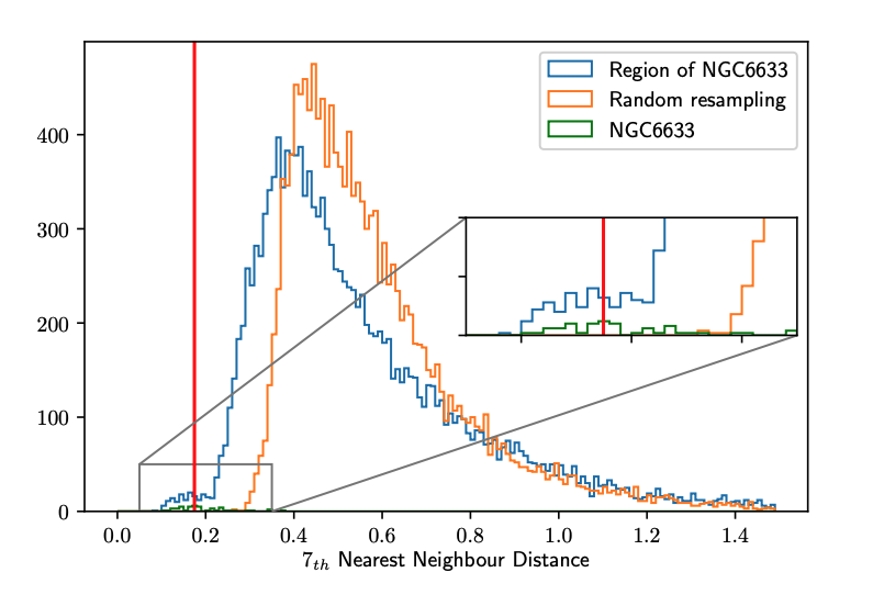
Fig. 3: Histogram of the 7th-NNDs of the region around the cluster NGC6633. The blue line shows the 7th-NND histogram of all the stars in that sky region in TGAS. Orange line shows the Green line shows the 7th-NND histogram for the listed members of NGC6633 (more visible in the zoom plot). The red line corresponds to the chosen value of in this region. The plot was made with the parameters L = 14 deg and minPts = 8. 7th-NND histogram of one realization of a random resample.
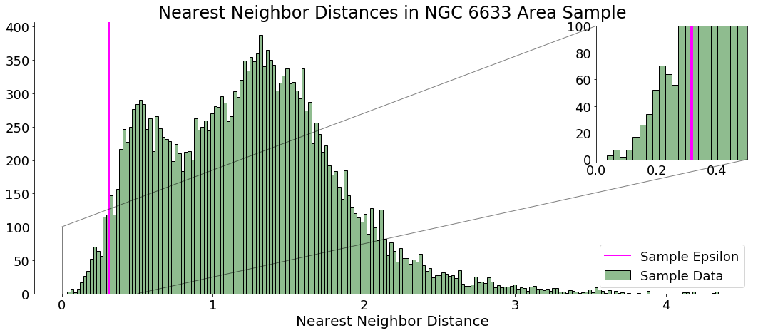
Compute (Sample )
I selected the 2.5th percentile value—the data point that is ~2 SDs from the mean—from my kNN histogram to be my values. I used this as a heuristic after several trial and error selections—the minimum value proved to be too stringent to detect clusters.
Compute (Simulated Gaussian Sampled Data Points)
Using sklearn’s KernelDensity function, I generated Gaussian KDEs for each parameter. I then simulated draws from these generated KDEs and used the sample draws as parameters for the Euclidian distance metric to compute the simulated kNN histogram.

With the Gaussian KDEs, I simulated sampling observations.
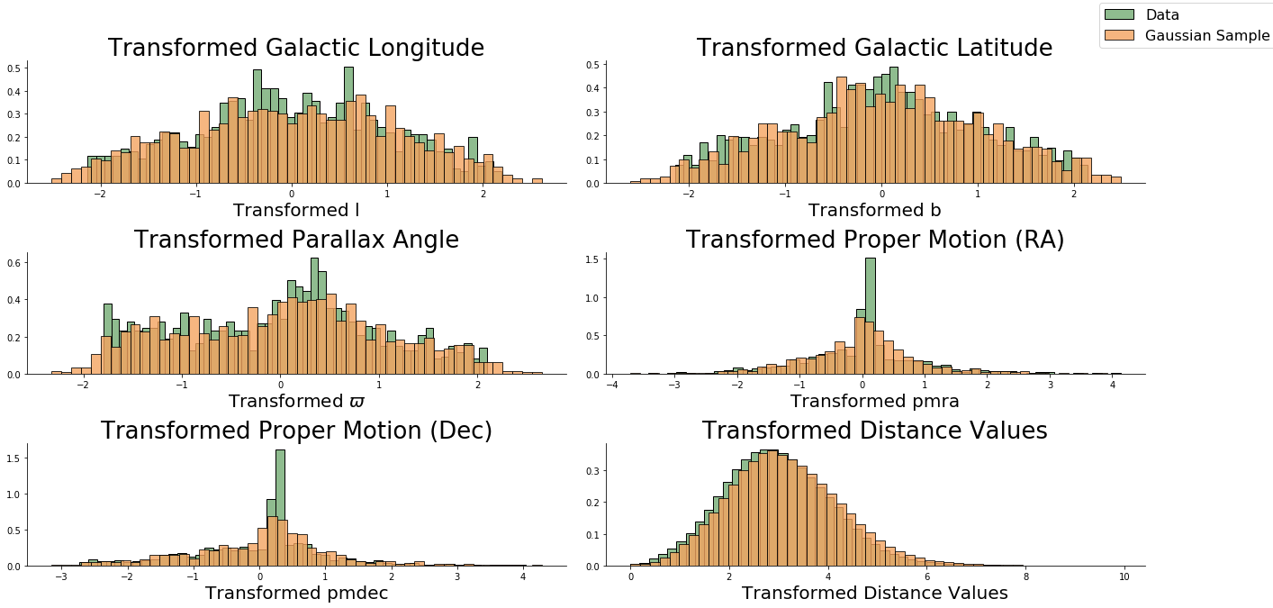
I then used the Gaussian KDE to generate multiple draws of kNN.
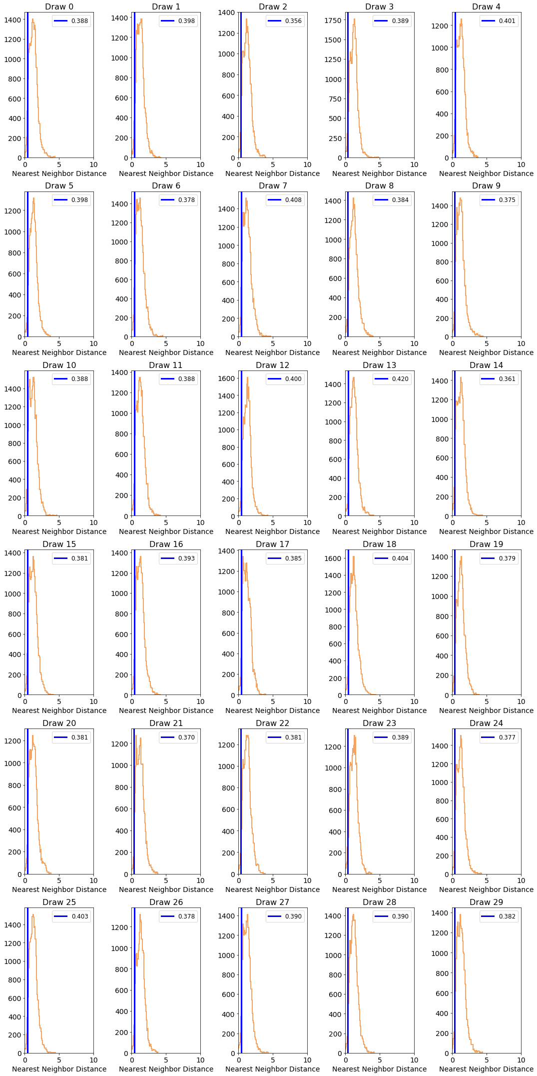
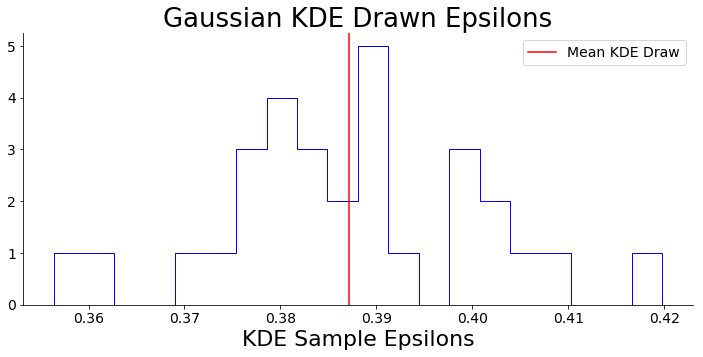
We can then perform the same kNN procedure for one random sample, plot the histogram of resultant kNN values, and estimate a value.
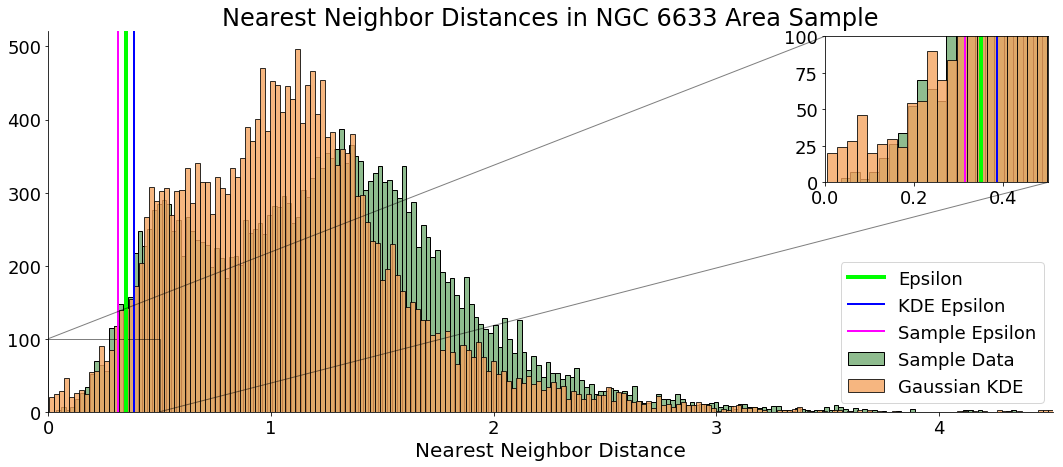
We now have an of ~0.351, which represents the maximum allowable distance between cluster members in degrees. I heuristically choose minPts to be 20, which means a cluster must have at least 20 stars.
Run DBSCAN on NGC 66333 Sample
With our transformed stellar observations, an value, and a minPts value, we can use sklearn’s DBSCAN cluster function and obtain cluster candidates for the portion of the sky we observe:
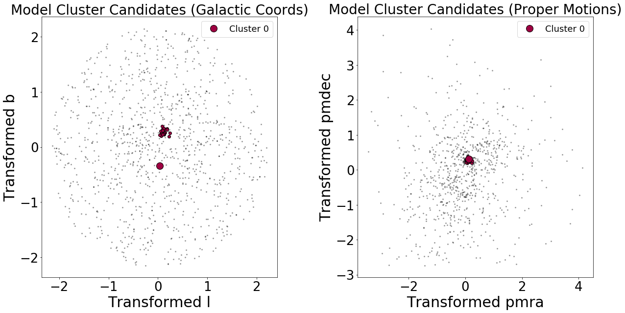
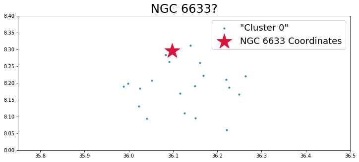
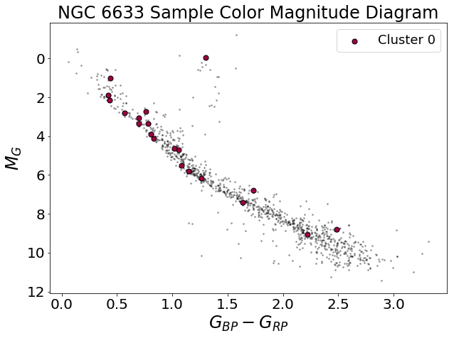
As a first pass, it seems this method works fairly well. DBSCAN correctly detected a cluster where the literature says there is a cluster. The procedure appears slightly inaccurate when it comes to determining cluster membership—NGC 6633 is reported to have a membership of about 30 stars, whereas the DBSCAN algorithm I implemented only finds 20 stars.
Modifying our value (by using a different “minimum”) or specifying a different minPts value could change these results:
- A larger means a more liberal distance criteria for cluster membership.
minPtsvalues determine how stringent we are with our definition of what constitutes a cluster.
We would also see different results if we used different pre-processing or a different distance metric.
Increasing Sample Size
I then increased the parameter space by widening the circle to 3 degrees instead of 1 degrees. The results of running the same analysis on our larger stellar sample:
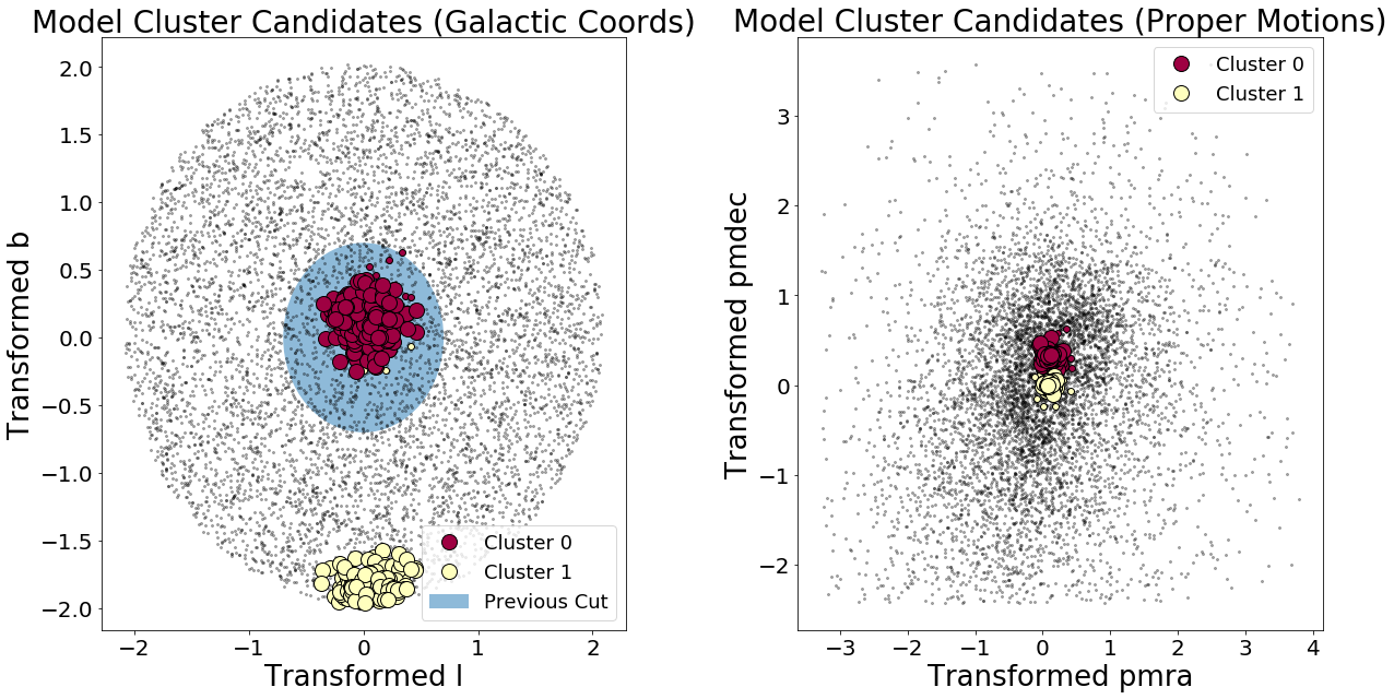
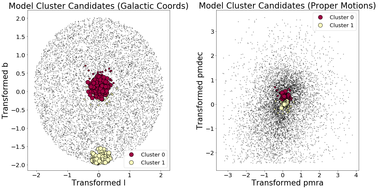
DBSCAN discovered two clusters!
It turns out that the second detected cluster is in the neighborhood of a reported stellar cluster, IC 4756!
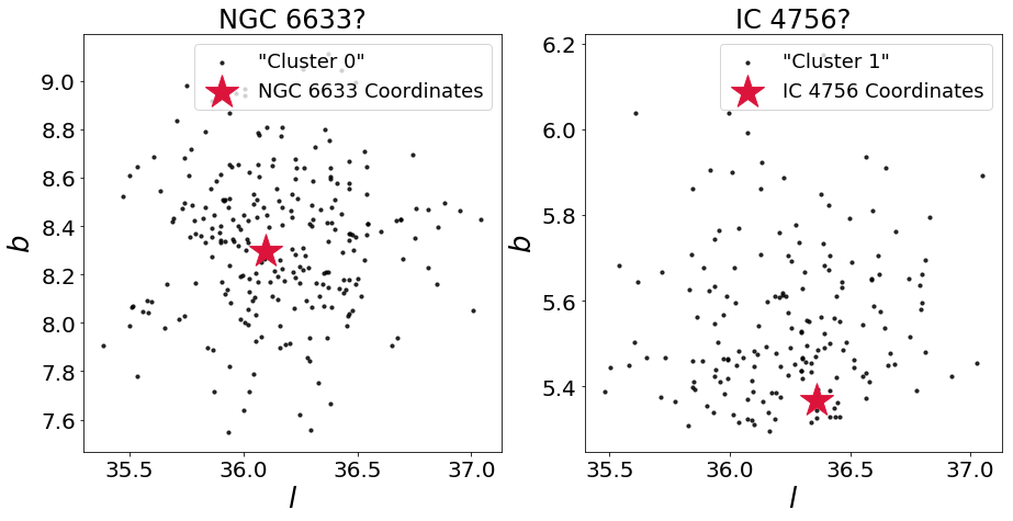
There’s a problem, however… The cluster size of “Cluster 0” has risen dramatically—from about 20 members to now 249 members. So we’ve detected clusters in the right location, but the algorithm needs some fine tuning when it comes to cluster membership.
Potential Improvements
Some considerations:
- Would increasing parameter space affect the way we’d want to normalize or power transform our data points?
- How does increasing parameter space affect our determination of ?
- Also, what’s going on with some of the Cluster 1 “members” appearing spatially far from Cluster 1’s core sample and encoaching on Cluster 0 territory in galactic coordinates?
The Distance Metrix
This deserves its own section, not just a bullet.
The Euclidian distance metric is a naive, simple model, but it is likely not the right distance metric to use—especially when we consider the parameters that get passed in (not just spatial coordinates, but angles and motion measurements). If you look closely, the metric combines units that do not work out—there are angles and frequencies mixed in with one another that should not be summed.
Many peculiarities, such as clusters that were close to one another in proper motion space but far in galactic coordinate space, could likely be solved by selecting a more appropriate distance metrix.
There are improvements to be made, for sure. If anything, this illustrates the challenge of choosing the right initial parameters for DBSCAN. That said, after this first pass, DBSCAN seems promising!
Now let’s take a look at Hyades with DBSCAN for fun.
DBSCAN Procedure on Hyades
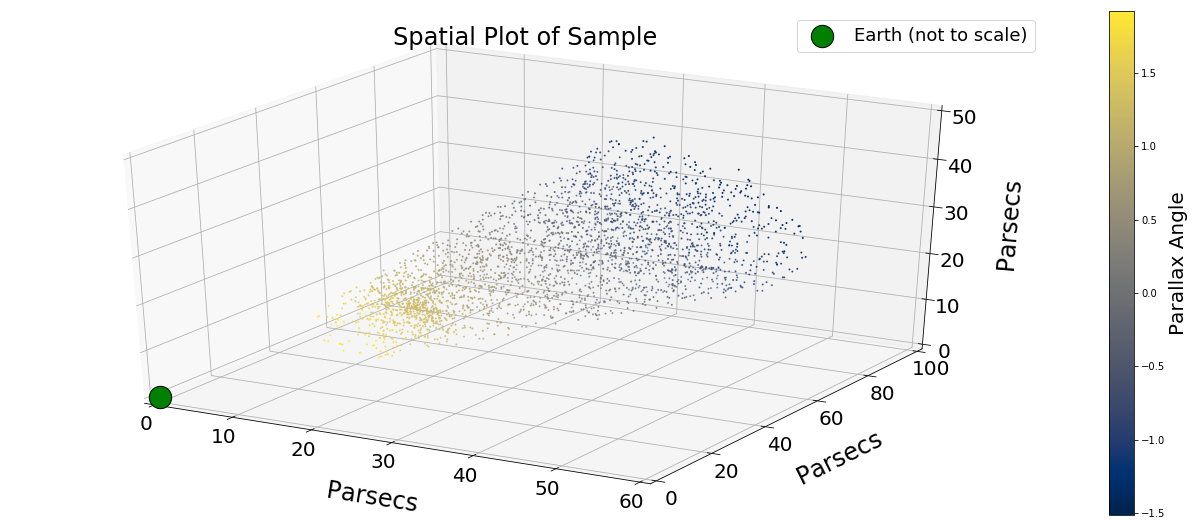
At the beginning of this report, I conducted a crude cylindrical cut of the sky to “detect” a star cluster. Let’s see what happens if we use DBSCAN to perform the same task.
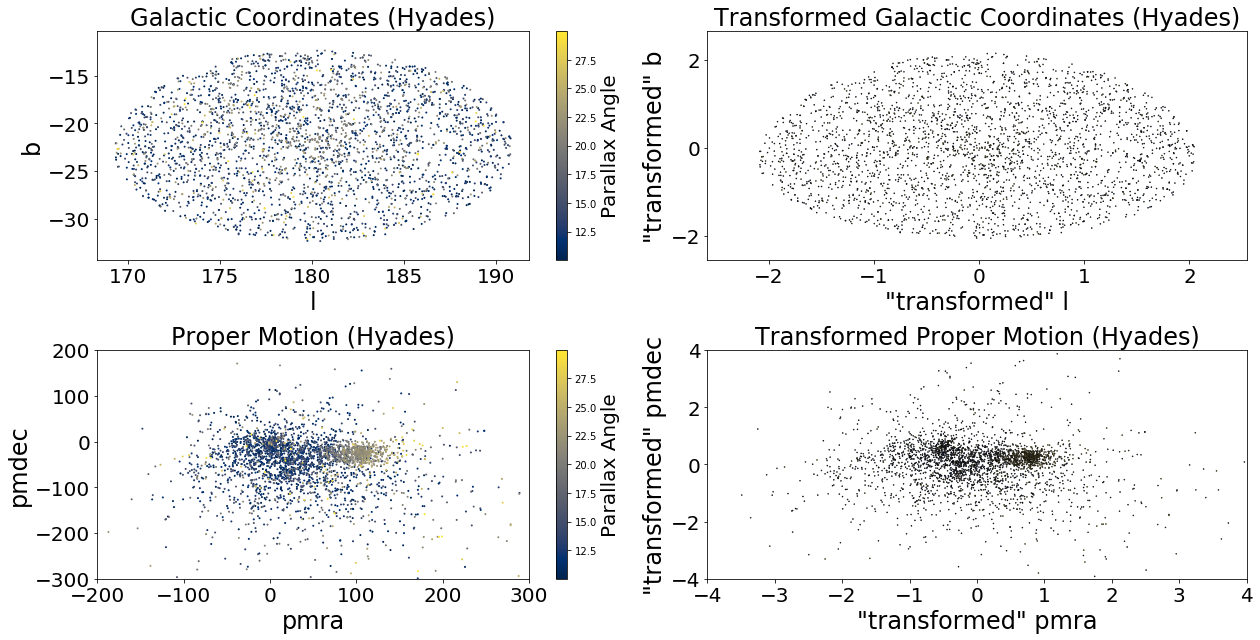
So we first acquire our sample:
Next, we compute for DBSCAN following the same procedure as before:
- As a prepatory step, standardize or normalize all values in the distance metric. For simplicity, ignore weights on the parameters.
- Compute the kth Nearest Neighbor Distance (kNND) histogram for each sample and save the “minimum value” as . Use domain knowledge to determine
minPtsand set . - Generate 30 random sample of stars using a Gaussian kernel density estimator, and then compute the kNND histogram for each sample and save each minimum value. The mean of all the minimum values is .
- Compute
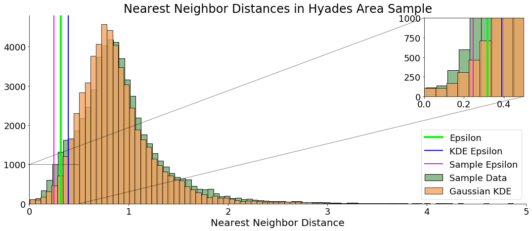
With and , we have the parameters we need to run DBSCAN on our sample:
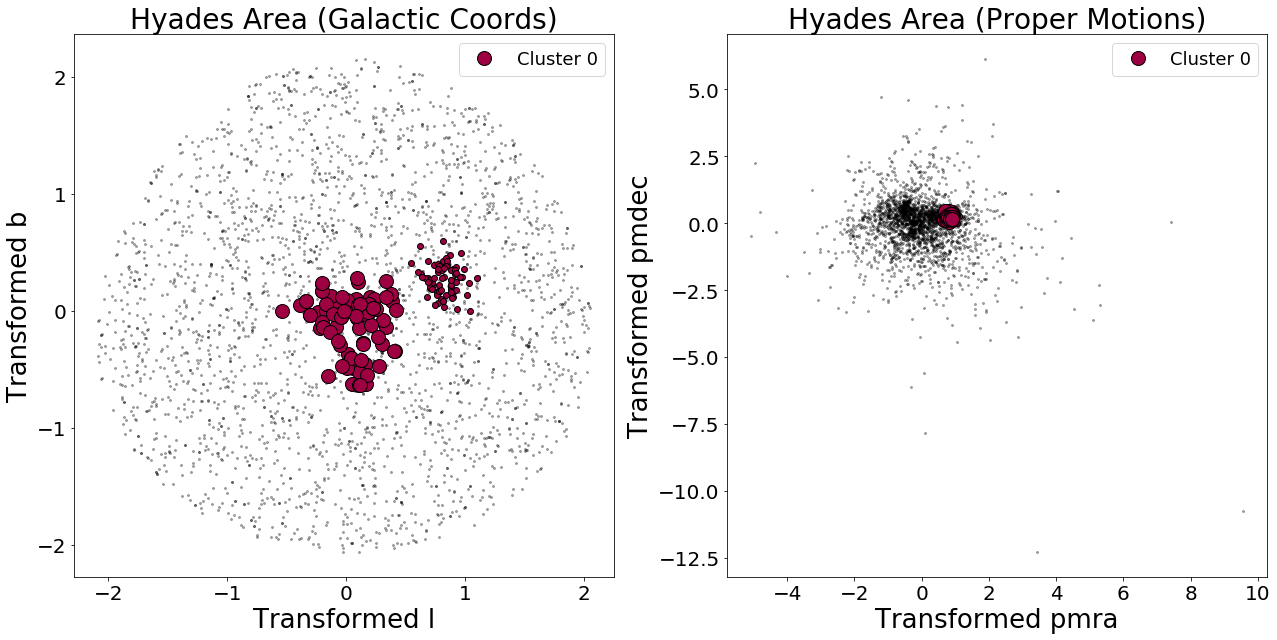
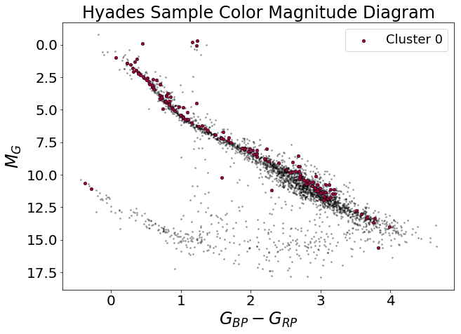
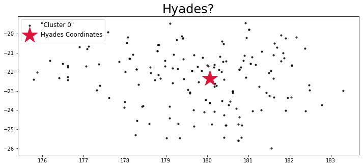
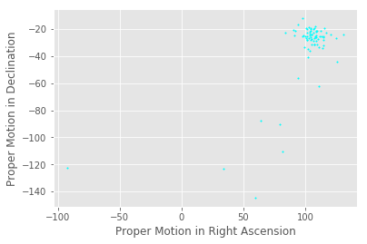
The algorithm is not perfect, but it appears to have worked fairly well! DBSCAN found a cluster where the literature says the Hyades cluster exists, and, to an order of magnitude, the number of cluster members is correct—the Hyades contains a few hundred stars, and DBSCAN found 163 stars.
After this, there are all sorts of improvements to be made:
- Applying Bayesian inference methods to improve on some parameter estimates, which we can treat as “priors”.
- Select a more appropriate distance function that properly accounts for spatial distribution and motion.
- Perhaps use a neural net to help with classification and candidate screening—they did this in the paper.
Still, for a first pass, not bad…