Standard Candle-Derived Period-Luminosity Relationship and Milky Way Dust Distribution

Alex | Last updated: February 28, 2019

This was a project I completed for UC Berkeley’s Astronomy Data Lab.

Goal

The goal was to build a dust msap of the Milky Way by deriving a dust distribution using the sample of RR Lyrae Stars curated by Gaia’s Data Relase 2 (Gaia DR2).

Scientific Backround: Using “Standardizable Candles”

RR Lyrae stars are periodic variable stars that can be treated as standard candles; RR Lyrae stars are special because they have a predictable brightness pattern that follow a period-luminiosity trend (the Leavitt law).

Measurements of periodicity and brightness allow for inferring intrinsic luminosity, which in turn allow for determining distances, which we can use to estimate color excess/extinction. All of the measured and derived quantities for the sample stars will ultimately help to create a map of the dust distribution in our Milky Way galaxy.

Method

An outline for the procedure I used to generate the dust map:

1. Obtained the relevant RR Lyrae data from Gaia Data Relase 2
2. Validated the pulsation period data by fitting light curves.
3. Obtained reported measurements for distances to RR Lyrae stars and associated apparent magnitudes, represented by mean G-band measurements.
4. Cleaned the data to ensure measured brightness is a function of distance alone.
5. Used the distance modulus to convert the distance and apparent magnitude measurements into absolute magnitudes.
6. Using Markov chain Monte Carlo, derived a Period-Luminosity linear model using the measured distances and computed absolute magnitude values.
7. Computed difference between luminosity values computed with the linear model and luminosity values derived from observed measurements.

I treated difference between the luminosity values computed by the linear model and the luminosity values derived from observed measurements as the extinction, or color excess. In astronomy, extinction is the absorption and scattering of light by dust and gas; if we assume that the amount of light that gets occluded from the observer is caused primarily by dust in between the observer and the star, then we can generate a temperature map of how much light was lost—effectively, a dust map.

Technologies

The project’s technical components included:

• Periodograms—Fourier decomposition

• Markov chain Monte Carlo

• Bayesian inference and modeling

• Data modeling and visualization The technologies involved in this project include:

• Python: IPython/Jupyter notebook, astroquery, pandas, matplotlib, numpy, matplotlib, scipy, emcee, corner, urllib, os

• ADQL: web database queries

Extracting RR Lyrae Data from Gaia Catalogs

The first step in this analysis is to obtain data for RR Lyrae candidates detected by Gaia; we want stellar parameters, light curves (flux versus time), and parallax measurements.

To fetch the data we seek and convert it into a usable datatable:

1. Query Gaia’s RR Lyrae catalogs, gaiadr2.vari_rrlyrae
2. Concatenate the resultant table with parallax measurements from gaiadr2.gaia_source, which will help us estimate distances.
3. Filter the table by selecting for targets that have valid pulsation frequency measurements. “Valid” means that a fundamental pulsation frequency (pf) has been measured had more than 40 clean epochs were obtained in the G-band.
4. Choose a sample size—I used a sample of 100 targets.
5. Transform the output to a pandas dataframe we can work with in Python.

Useful documentation for column labels, RR Lyrae parameters/derivations, and data querying syntax:

• Documentation for Gaia DR2’s RR Lyrae star table
• Individual column labels
• RR Lyrae parameters and derivations
• Querying Gaia data with Astroquery

Why G-band Magnitude?

The G-band is one of the photometric bands used in the Gaia mission to measure the brightness of stars. It is particularly valuable because it covers a wide range of wavelengths in the optical spectrum, making it useful for determining the overall brightness of stars.

The mean G-band magnitude represents the average brightness of the star in the G-band filter; it provides a single number that characterizes a star’s typical luminosity and can be used to estimate a star’s absolute magnitude (luminosity) when combined with distance information (parallax).

Gaia DR2 provides individual photometric measurements; calculating the mean magnitude is a post-processing step that we have to do. Note that the measurement values of magnitudes are logarithmic quantities, so some numerical conversions are needed in the calculation process.

Obtaining Periodicity and G-band Brightness

Gaia’s vari_rrlyrae catalog includes calculated pulsation periods and G-band magnitude values for each star. These values can be used to obtain distance estimates.

Period Data Reliability Check

To assess the reliability of values reported in the Gaia catalog, I generated my own estimates of the pulsation periods.

The process I used to estimate periods:

1. Download raw light curves for the sample stars.
2. Fit and fold the light curves using periodograms to determine pulsation frequnecies.
3. Compare my pulsation period estimates with Gaia DR2’s reported values.

1. Download Raw Light Curves

I used Python’s urllib package to download the raw, unfitted light curves that correspond to the 100-target sample downloaded above.

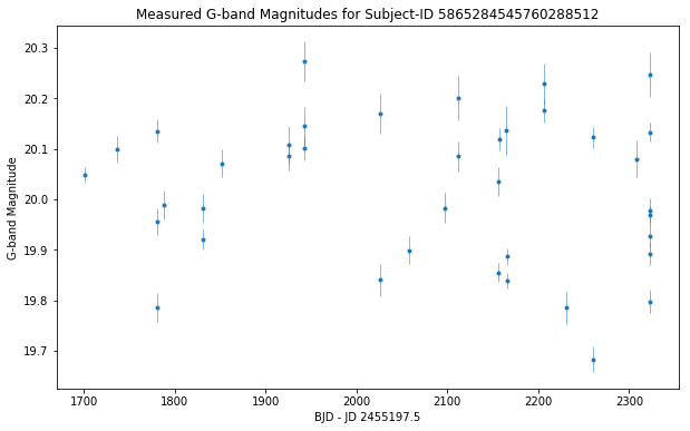
2. Estimate Pulsation Frequencies Using Periodograms

With this raw data in hand, I used the AstroPy implementation of the Lomb-Scargle periodogram to estimate pulsation periods. (The fit generated from this implementation also contains a mean magnitude calculation.)

Periodograms are statistical tools used to identify periodic patterns in unevenly sampled time-series data. The Lomb-Scargle periodogram takes in a star’s time-series brightness data and associated error estimates, tests for periodic signals, and determines the peak/dominant frequency signal—this dominant signal is what I considered the fundamental pulsation frequency of a given star.

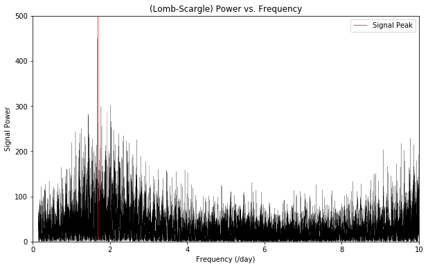
3. Compare My Estimates With Gaia DR2’s Reported Values

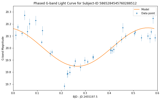
My light curve-derived period estimates followed the general trend of the data points provided by Gaia DR2. For a more rigorous comparison between the derived and reported data values, I computed a basic percent error and visualized the calculation with a histogram—I “accepted” any data points within 100% error, since errors in astronomical measurements are often… astronomical.

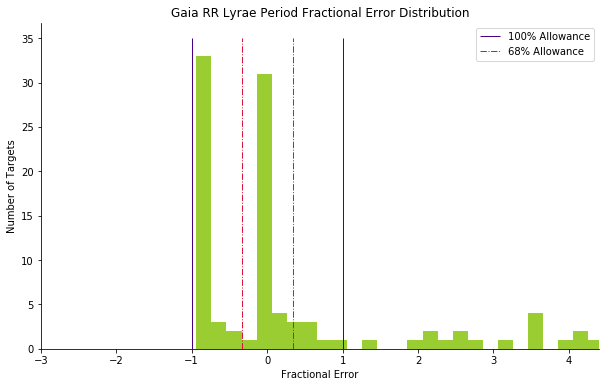
The Lomb-Scargle-generated model does a decent job capturing the data:

• With a 100% error acceptance range, 76% of targets “match” the Lomb-Scargle- generated models.
• With a more stringent, classical 68% error (1 standard deviation) acceptance range, almost half of the observed targets match the Lomb-Scargle-generated model curves.

Admittedly the 1 standard deviation range isn’t great… To minimize error, one can use different Lomb-Scargle normalization methods, which would result in different period estimates. Leveraging bootstrapping, or treating sample statistics as population parameters, may also help to generate a better fit.

Overall, I was satisfied with this quick sanity check.

Absolute Magnitudes

To infer a period-luminosity relation, we can use absolute magnitude as a measure of luminosity.

In astronomy, the brightness of a distant object can be measured in two ways:

• Absolute magntiude, which is a measure of how bright an object would be if it were seen from a standard distance (10pc). It is an intrinsic brightness measure—brightness that is normalized against and hence does not depend on distance.
• Apparent magnitude, which is a measure of how bright the object appears as is. In short, the more distant the object, the less bright it appears.

The distance modulus is a formula that relates absolute magnitude and apparent magnitude; if we know the distance and the apparent magnitude, we can obtain the absolute magnitude.

Fortunately, we have apparent magnitude from Gaia DR2 and distance estimates from the Bailer Jones catalog.

Distance Measurements in Gaia DR2

We can make naive distance estimates in astronomy using the following equation:

$d = 1/p$

where d is the distance to the star in parsecs and p is the parallax angle in arc seconds.

However, if we use this estimate, we’ll find that there are large deviations from the distance values reported in Gaia DR2;

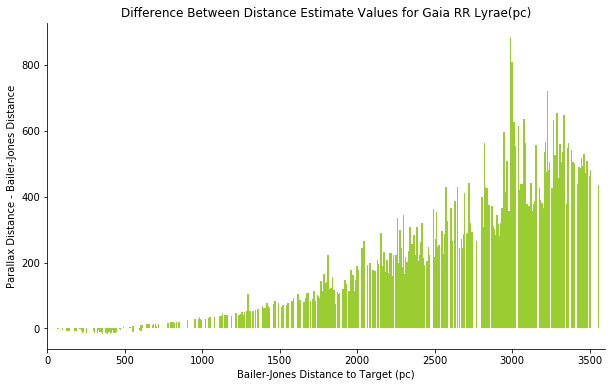
The Bailer-Jones catalog includes distance measurements that were derived using statistical methods that account for factors that the naive distance estimate ignores, including:

• Uncertainties and error propagation in the measured parallax measurements
• Correlations accounting for proper motions, stellar coordinates, and errors in positional measurements
• Systematic errors and potential biases from the spacecraft, data processing software, and astrometry design
• Completeness of the dataset—astronomers estimated a selection function to account for severe biases

Naturally, I used the more rigorous Bailer-Jones distance measurements to derive absolute magnitude estimates.

Data Cleaning

Removing Dust for Distance Modulus

In order to use absolute magnitude estimates derived from the distance modulus, I had to select appropriate data points.

The distance modulus provides a relationship between absolute magnitudes, distances, and apparent magnitudes; the formula treats the dimming of light as a function of distance alone and does not account for any other physics—most prominently, it does not account for the photon scattering effects of dust particles that lie between observers and distant stars.

The presence of dust would lead to the distance modulus underestimating absolute magnitude values. For this reason, in order to reliably use the distance modulus, it was important to select targets that were not significatly occluded by dust.

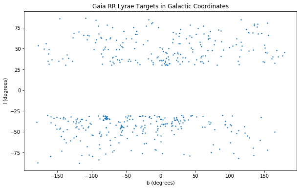
Fortunately, we know that the vast majority of the dust in the Milky Way exists near the galactic plane—one can think of this as our galaxy’s disc.

To avoid having to account for dust in calculations to derive distances, I selected targets from Gaia DR2 that have relatively accurate distance measurements, are above or below the disk by at least 30 degrees, and are relatively nearby (within 4kpc).

Removing Noisy Data Points

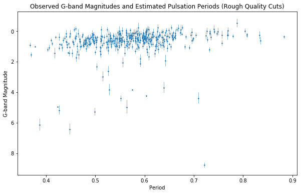
Gaia DR2 also reports excess noise and error factors, such as astrometric_excess_noise, phot_bp_rp_excess_factor, and astrometric_n_good_obs_al.

I applied the same data quality cuts for several paramters as Lindegren et al. 2018 to the target sample.

Removing Outliers With Naive Parameter Approach

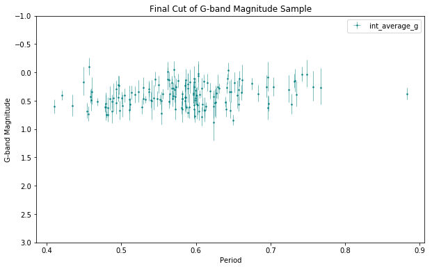
For a last data cut before fitting a linear relation between period and luminosity, I restricted the range of allowable metallicity and mean magnitude values to remove remaining outliers.

Fitting a Linear Relation Between Period and Luminosity Using MCMC

Now that we have filtered our sample through various data quality checks, we are ready to attempt a fit.

For a linear relation, let’s assume:

$M_G=a×log[P/day]+b$

where

• $M_G$ is the absolute magnitude of a star
• $P$ is the RR Lyrae period
• $a$ and $b$ are parameters that we will estimate.

Instead of using least-squares regression, where error measurements are assumed to be correct, Gaussian, and independent—an incorrect assumption for our data—I used Markov chain Monte Carlo (MCMC) to fit a linear model to the data.

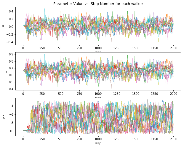
To do this, I initialized log-likelihood, log-posterior, and log-prior functions that take into account observations and observation error ranges. I also initialized a few guess parameters for a and b.

To obtain priors for our MCMC process, I used the guess parameters and scipy’s minimize function to generate a best fit using the log likelihood function.

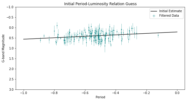
Using the priors, the observed data points, the error estimates for each data point, and the aforementioned log functions, I used functions provided by the emcee package in Python to generate a best-fit line.

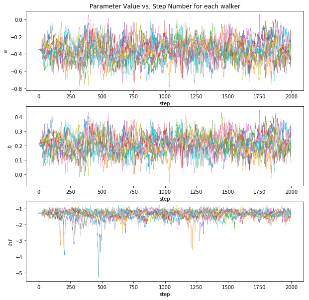
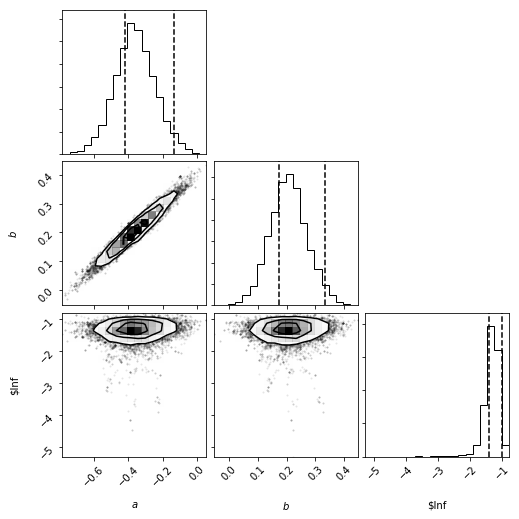
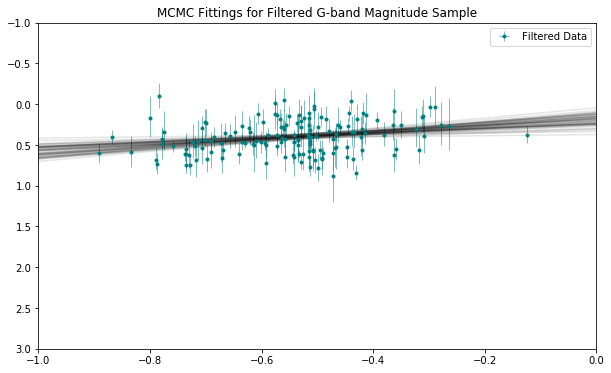
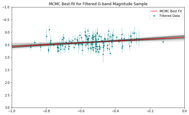
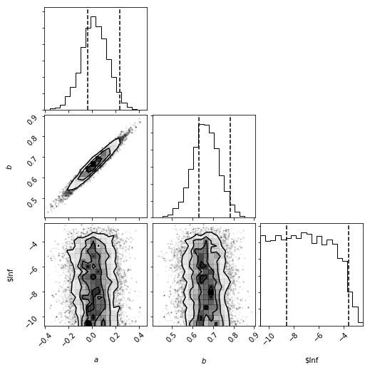
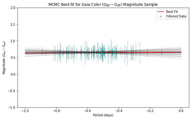
The MCMC process suggests that a is -0.36 and b1 is 0.21. As this is astronomy, I round liberally to obtain the following Period-Luminosity relation:

$M_G≈−0.4×log[P/day]+0.2$

In theory, this relationship allows us to compute the absolute magnitude—or intrinsic brightness—of a star.

For the purposes of this project, we can calculate the intrinsic brightness from observed periods and then use the distance modulus to compute the apparent magnitude—the brightness of the star we would expect to observe, if distance was the only factor in diminishing brightness. In effect, we can remove the effects of distance and treat any additional dimming as an effect of another physical phenomena —dust!

How cool!

Period Extinction Relation

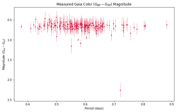
We now have a statistical process whereby we can take in Gaia DR2’s RR Lyrae distance and magnitude data and obtain a reasonable linear model describing a relationship between distance and magnitude.

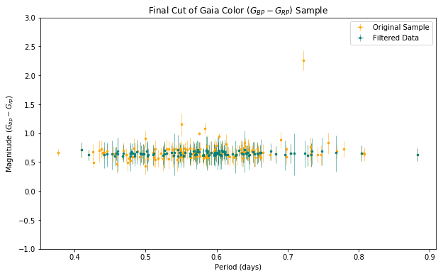
Gaia DR2 helpfully provides magnitudes for specific color ranges.

I performed the same data quality cuts and MCMC process to derive a period-luminosity relation for the $G_{BP} - G_{RP}$ color band.

Dust Map

Now that we have obtained a Period-Luminosity relationship, for each RR Lyrae star in Gaia DR2, so long as the data is populated—measurements exist for parallax and relevant G-band magnitudes—we can calculate the color excess or extinction:

$E(G_{BP}−G_{RP})=(G_{BP}−G_{RP})_{observed}−(G_{BP}−G_{RP})_{intrinsic}$

where

• $(G_{BP}−G_{RP})_{observed}$ represents the measured magnitude reported by Gaia DR2
• $(G_{BP}−G_{RP})_{intrinsic}$ represents the “real” magnitude value assuming my MCMC model is correct.

Again, the MCMC-derived Period-Luminosity relationship can be used to remove the effects of distance on the dimming of brightness from an observed star. Any additional dimming—represented by color excess here—I considered to be a result of dust scattering starlight.

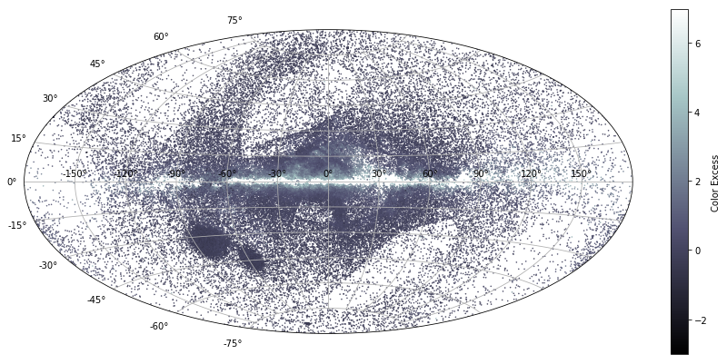
I plotted the resultant color extinction values using SkyCoord and an Aitoff projection (a modified map projection) in the galactic frame. The resultant temperature map essentially maps estimates for the locations and densities of dust in the Milky Way galaxy.

How does this compare to values reported by the pros? We can plot “official” values by using the dustmaps package and calling dustmaps.sfd. Take a look at the result:

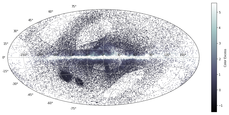
Wow… That’s pretty darn close! How cool!

To make a quantitative comparison between the two dust maps, I couldn’t do a simple subtraction of the values because the values that generated my dust map versus the values that generated dustmaps’ were measured in different wavelengths.

Qualitatively, though, the sfd plot and my derived extinction plot agree on the overall distribution of dust in our galaxy. However, it’s clear that the sfd plot shows greater densities of dust across the board.

The discepancy makes sense. The sfd values originate from a more rigorous approach than mine. My approach only “sees” dust between RR Lyrae targets and an observer—the sfd values “see” dust well past the RR Lyrae targets.